1. Preparing and submitting your gene/protein sets
TopoGSA accepts lists of genes, proteins or microarray probe-identifiers as input. These lists of identifiers are mapped onto a molecular interaction
network by first converting the identifiers into the gene/protein name format of the network (if necessary) and then identifying which
of the molecules are present in the network. To guarantee a successful conversion process, the identifiers should have one of the following formats
(depending on the species under consideration):
Please make sure to choose the correct format for your dataset from the drop-down menu
"Species and identifier format" on the start page.
If you would like to analyse an example dataset first, you can select one of the options from the
"Insert example data" menu. In this tutorial we will use the first option, the comprehensive set of human cancer genes (Futreal et al., 2004), as example.
Fig. 1 shows the correct settings on the web-interface for this dataset (for all examples the settings are configured automatically).
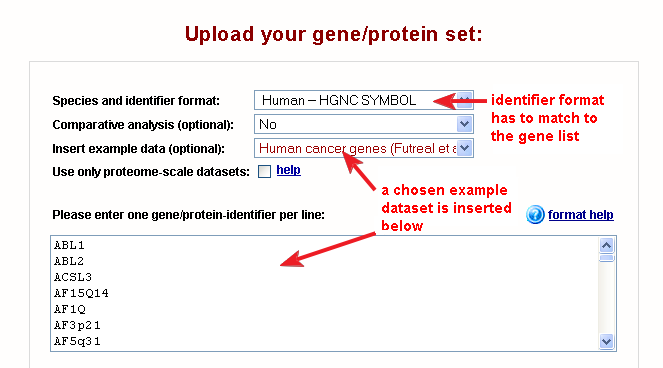 |
| Fig. 1: web-interface settings for the human cancer genes example dataset |
To upload your own dataset, please insert only one gene/protein identifier per line and use the same identifier format for each entry (automatic disambiguation of homonyms is not supported). The maximum allowed dataset size is 1000 genes or proteins (larger datasets would cover major parts of the interaction network and would not be suitable for comparison against much smaller reference datasets).
Optionally, you can assign class labels to the identifiers in order to group subsets of genes
together (data points with the same class label will receive the same colour when plotting the results). For this purpose, arbitrary class labels
(e.g. "tumour"/"normal", "class1"/"class2"/"class3") can be written behind the gene/protein names, separated by a comma. For example,
ENSG00000002016,tumour
ENSG00000005339,tumour
ENSG00000005339,normal
ENSG00000134058,normal
ENSG00000010704,tumour
...
would be a valid gene set with class labels to be mapped on a human interaction network (to view a real-world example with class labels, you can select the 'Microarray, two classes' dataset from the example data menu).
Before submitting a dataset and also during a gene/protein set analysis the user can always switch between two analysis types:
If you wish to skip the individual dataset analysis (the default first step), you can directly submit your dataset to the comparative analysis, by choosing an option from the
"Comparative analysis" menu on the main interface (see
Fig. 1). For the human species, the available reference datasets include gene/protein sets from KEGG and BioCarta signalling pathways, Gene Ontology and InterPro (for non-human species, the reference datasets are extracted from the Gene Ontology and/or the MetaCyc database)).
Human gene or protein lists can be mapped onto two alternative human protein interaction networks:
To use the second network above, simply activate the check-box
"Use only proteome-scale datasets" on the main interface (see
Fig. 1).
To submit your dataset, click on the
"Start analysis" button. Instructions on how to use alternative analysis types can be found in section 5 (
Using microarray data as input) and 6 (
Using your own interaction network as input).
2. Checking gene/protein name conversion and network mapping
After submitting a dataset, the user will first be presented with conversion and mapping summary, revealing which genes or proteins from the uploaded list could successfully converted into a standard identifier format and were present in the interaction network for the chosen species (human, yeast, fly, plant or worm). For the human cancer genes example data set, the first entries of the resulting conversion and mapping table are shown below:
| original identifiers |
converted identifiers |
present in network |
| ABL1 |
ENSG00000097007 |
yes |
| ABL2 |
ENSG00000143322 |
yes |
| ACSL3 |
ENSG00000123983 |
yes |
| AF15Q14 |
not found |
no |
| ... |
... |
... |
By clicking on the column titles, you can sort each column alphabetically and quickly identify whether a specific gene/protein in the uploaded list could not be converted to the standard format in the network (in the example above: from HGNC SYMBOL format to ENSEMBL format, e.g. the human cancer gene AF15Q14 could not be converted), or whether the corresponding molecule is not present in the network (see last column). If none of the input identifiers
could be converted successfully, the system will attempt to detect the identifier format automatically. If this automatic identification process fails, the user will be notified. The submitted gene list and the selected identifier type will be shown to help the user in solving problems related to the input format.
3. Analysing topological properties of genes/proteins in your dataset
In order to obtain a first general overview on the network topological properties of the uploaded gene/protein set, the first outcome
is a statistics table, providing the user with the averaged values for five topological properties (shortest path length centrality, node betweenness, node degree, local clustering coefficient and eigenvector centrality) computed for the uploaded gene set, 10 matched-size random gene sets in the network (as a random model) and for the entire network. As example, the output for the human cancer genes example dataset is shown below (see
Tab. 1).
| Shortest path length | Node betweenness | Degree | Clustering coefficient | Eigenvector centrality |
|---|
| Uploaded gene/protein set | 3.74 | 54460 | 21.37 | 0.1 | 0.05 |
|---|
| 10 random simulations (mean) | 4.84 (±0.04) | 5052 (±764) | 3.97 (±0.26) | 0.02 (±0) | 0.03 (±0) |
|---|
| Static mean over entire network | 4.12 (±0.94) | 14669 (±68893) | 8.27 (±16.2) | 0.11 (±0.21) | 0.02 (±0.04) |
|---|
|
| Tab. 1: general topological statistics for the human cancer genes example dataset, a random model and the entire network |
In this table, the user can for example see that the average node betweenness and degree of the uploaded gene set exceed the corresponding values for the matched-size random gene sets by several standard deviations. Please note that the topological properties are not necessarily normally distributed, and care must be taken when interpreting these averaged results: The user should additionally check the 2D and 3D plots of the topological properties (see below), to determine whether the dataset contains outliers.
The different network topological properties of genes/proteins from the uploaded dataset can be plotted and visualized. To investigate other pairs or triples of topological properties in the 2D- and 3D-plots, the user can select a property of interest for each coordinate (X- Y- and optionally Z-axis) and click on the
"Regenerate gene set plot" button.
Moreover, before regenerating the plots, a filtering can be applied to each property, in order to remove data points below a given percentile threshold. As an alternative to the filtering option, the user might prefer to use the in-built zooming feature in the 2D and 3D plots. All plots are interactive and allow the user to zoom into the plot by using the mouse wheel (or left-click on empty areas in the 2D plot and Shift + left-click in the 3D plot) and obtain functional annotations for the plotted genes/proteins, by clicking on the corresponding data points. An example 2D plot for the human cancer genes dataset by Futreal et al. (2004) is shown below (see
Fig. 2) and also provides the interactive zoom- and annotation-features mentioned above). In this 2D example plot, one can clearly see that the tumour suppressor gene P53 (symbol: TP53) has outstanding network properties (a high node betweeness and a small shortest path length centrality) in comparison to the other genes in the dataset.
The 2D and 3D visualizations of the topological features for each single molecule in the gene/protein set also enable the user to compare coloured sub-groups of identifiers, if the user has provided class labels for the uploaded dataset (see
Section 1).
zoom out 1.0 2.0 3.0 4.0 5.0 6.0 7.0 0 250000 500000 750000 1000000 1250000 1500000 1750000 2000000 2250000 |
|
|
| Fig. 2: Interactive 2D topological properties plot for the human cancer genes example dataset. Here, the node betweenness is plotted against the shortest path length (use left mouse-click or scroll-wheel to zoom into the plot, hover mouse over data points to see annotation data) - below the corresponding 3D plot is shown (Java-enabled browser required) |
The 3D-plots are available in two different formats to ensure compatibility with the user's system (for Java-enabled browsers, the LiveGraphics3D plot can be used; otherwise, free VRML-browser plug-ins can be used to explore the data in a VRML-environment).
4. Comparing your dataset to reference datasets
By clicking on the
"Compare to existing datasets" button at the bottom of the individual dataset analysis page or by selecting a reference database in the
"Comparative analysis" menu on the start page, the user can compare an uploaded gene/protein set against a collection of reference datasets. These reference gene/protein sets represent cellular pathways and processes, molecular functions or sub-cellular localisations and have been collected from public annotation databases including KEGG, Gene Ontology, BioCarta, InterPro and MetaCyc. For the human species reference gene sets are available from each of these databases, except the MetaCyc database, and for other species, the reference datasets were obtained from the Gene Ontology database and/or MetaCyc.
TopoGSA provides two possibilities to compare the topological properties of these reference datasets against the uploaded dataset:
In analogy to the previous individual dataset analysis, interactive 2D and 3D plots are also available for the comparative analysis. However, since there are many reference gene sets with large sizes, only the median values of their topological properties are plotted to prevent overcrowded plots.
Fig 3. below shows a 2D comparative plot for the human cancer genes example dataset in comparison with datasets from the KEGG database. The KEGG datasets are coloured based on the top-level hierarchy of the KEGG-BRITE categorization of cellular pathways to facilitate the distinction between different types of pathways. Just as for the plots in the individual dataset analysis, the user can zoom into the plot with the mouse (using the mouse-wheel or left-click into empty regions) and see labels by hovering the mouse over data points. Moreover, the user can highlight data points by clicking on them and the corresponding entries in the similarity ranking table below will be highlighted in red text colour.
zoom out 0.0 1.0 2.0 3.0 4.0 5.0 0 250000 500000 750000 1000000 1250000 1500000 1750000 2000000 2250000 | Metabolism | | Genetic Information Processing | | Cellular Processes | | Environmental Information Processing | | Human Diseases | | uploaded gene set (median) | | uploaded gene set (all) |
|
|
|
| Fig. 3: Comparative plot for the human cancer genes example dataset in combination with KEGG gene sets (this is an interactive plot, which has been "zoomed" to an interesting region) - below the corresponding 3D plot is shown (Java-enabled browser required) |
In addition to this qualitative comparison of topological properties, the similarity ranking table (see
Tab. 2 below) provides a quantitative comparison of the uploaded dataset with the reference datasets, based on a similarity score (given in the last column of the ranking table).
The similarity score is obtained by computing 5 ranks for each pathway/process set according to the absolute diffences between each of its 5 median topological properties and the corresponding value for the uploaded gene/protein set. The sum of ranks across all topological properties is then computed and normalized to a range between 0 and 1. As with previous data tables, each column can be sorted alpha-numerically by clicking on the corresponding column-header.
Moreover, the user can identify whether datasets are topologically similar due to a large overlap between their genes or proteins, in the column displaying the number of genes in the gene sets (2nd column from the right), the size of the overlap between the reference gene sets and the user-defined gene set is shown in brackets.
[Legend: CC = clustering coefficient; SPL = shortest path length; BW = betweenness; EVC = eigenvector centrality]
| Identifier | Median
degree | Median
CC | Median
SPL | Median
BW | Median
EVC | No. of
genes | | uploaded gene set | 10 | 0.07 | 3.67 | 9895 | 0.02 | 311 |
Identifier  | Median degree | Median CC | Median SPL | Median BW | Median EVC | No. of genes | Score | | hsa04120:Ubiquitin mediated proteolysis | 9 | 0.05 | 3.68 | 11949 | 0.02 | 105 (11) | 0.09 | | hsa04530:Tight junction | 10.5 | 0.04 | 3.67 | 9686 | 0.02 | 106 (11) | 0.1 | | hsa04010:MAPK signaling pathway | 12 | 0.05 | 3.64 | 9390 | 0.03 | 225 (22) | 0.11 | | hsa04810:Regulation of actin cytoskeleton | 13.5 | 0.05 | 3.65 | 11277 | 0.02 | 184 (19) | 0.11 | | hsa04650:Natural killer cell mediated cytotoxicity | 11 | 0.04 | 3.66 | 7169 | 0.02 | 117 (11) | 0.12 | | hsa04150:mTOR signaling pathway | 14.5 | 0.07 | 3.64 | 14883 | 0.02 | 48 (8) | 0.12 | | hsa04310:Wnt signaling pathway | 10 | 0.04 | 3.76 | 9607 | 0.01 | 123 (9) | 0.13 | | hsa04540:Gap junction | 12 | 0.03 | 3.67 | 12696 | 0.02 | 79 (10) | 0.14 | | hsa04512:ECM-receptor interaction | 10 | 0.06 | 3.83 | 6407 | 0.01 | 73 (1) | 0.15 | | hsa04912:GnRH signaling pathway | 14 | 0.04 | 3.65 | 11884 | 0.02 | 82 (8) | 0.15 | | hsa04350:TGF-beta signaling pathway | 14 | 0.05 | 3.63 | 15594 | 0.02 | 82 (4) | 0.16 | | hsa05030:Amyotrophic lateral sclerosis (ALS) | 7 | 0.05 | 3.7 | 2244 | 0.02 | 19 (2) | 0.16 | | hsa04910:Insulin signaling pathway | 14 | 0.07 | 3.58 | 14485 | 0.03 | 123 (16) | 0.17 | | hsa05020:Parkinson's disease | 9 | 0.03 | 3.74 | 13520 | 0.01 | 20 (0) | 0.17 | | hsa04330:Notch signaling pathway | 15 | 0.08 | 3.59 | 11534 | 0.03 | 40 (5) | 0.18 | | hsa04916:Melanogenesis | 10 | 0.03 | 3.82 | 11500 | 0.01 | 80 (13) | 0.19 | | hsa04630:Jak-STAT signaling pathway | 7 | 0.12 | 3.7 | 7817 | 0.03 | 132 (23) | 0.19 | | hsa04510:Focal adhesion | 15 | 0.06 | 3.55 | 14237 | 0.03 | 181 (23) | 0.2 | | hsa04730:Long-term depression | 14 | 0.04 | 3.74 | 14665 | 0.01 | 68 (7) | 0.21 | | hsa04670:Leukocyte transendothelial migration | 16 | 0.05 | 3.57 | 13395 | 0.03 | 99 (7) | 0.21 | | hsa04360:Axon guidance | 7 | 0.03 | 3.82 | 6892 | 0.01 | 111 (7) | 0.21 | | hsa04950:Maturity onset diabetes of the young | 7.5 | 0.02 | 3.81 | 6535 | 0.01 | 18 (0) | 0.22 | | hsa04720:Long-term potentiation | 15 | 0.04 | 3.58 | 15945 | 0.03 | 63 (8) | 0.24 | | hsa04620:Toll-like receptor signaling pathway | 15 | 0.09 | 3.56 | 14237 | 0.03 | 89 (6) | 0.24 | | hsa04640:Hematopoietic cell lineage | 8 | 0.1 | 3.9 | 5120 | 0.01 | 82 (3) | 0.25 | | hsa01430:Cell Communication | 6 | 0.07 | 3.92 | 3483 | 0.01 | 84 (1) | 0.26 | | hsa04514:Cell adhesion molecules (CAMs) | 6 | 0.06 | 3.98 | 5330 | 0.01 | 109 (1) | 0.27 | | hsa04610:Complement and coagulation cascades | 8 | 0.06 | 3.99 | 4951 | 0 | 67 (0) | 0.27 | | hsa04070:Phosphatidylinositol signaling system | 5 | 0.01 | 3.76 | 2117 | 0.01 | 55 (3) | 0.28 | | hsa04020:Calcium signaling pathway | 6 | 0.04 | 3.9 | 2952 | 0.01 | 151 (6) | 0.31 | | hsa04940:Type I diabetes mellitus | 7 | 0.06 | 4.2 | 7169 | 0 | 43 (2) | 0.31 | | hsa05010:Alzheimer's disease | 16 | 0.05 | 3.63 | 24871 | 0.02 | 28 (0) | 0.32 | | hsa03022:Basal transcription factors | 13.5 | 0.15 | 3.8 | 4467 | 0.01 | 28 (0) | 0.33 | | hsa04060:Cytokine-cytokine receptor interaction | 6 | 0.09 | 4.01 | 3507 | 0.01 | 216 (14) | 0.33 | | hsa04115:p53 signaling pathway | 21 | 0.07 | 3.57 | 18855 | 0.02 | 59 (14) | 0.34 | | hsa04740:Olfactory transduction | 4.5 | 0 | 3.95 | 6329 | 0.01 | 20 (0) | 0.35 | | hsa00240:Pyrimidine metabolism | 5 | 0.04 | 3.88 | 1523 | 0 | 53 (0) | 0.35 | | hsa04710:Circadian rhythm | 9 | 0.17 | 3.87 | 5787 | 0.01 | 12 (1) | 0.35 | | hsa05217:Basal cell carcinoma | 6 | 0.05 | 4.11 | 5875 | 0 | 43 (5) | 0.35 | | hsa05211:Renal cell carcinoma | 16.5 | 0.07 | 3.51 | 16292 | 0.04 | 66 (17) | 0.37 | | hsa00860:Porphyrin and chlorophyll metabolism | 3 | 0 | 3.89 | 11162 | 0.01 | 13 (0) | 0.38 | | hsa04140:Regulation of autophagy | 4 | 0.02 | 3.93 | 2742 | 0.01 | 17 (0) | 0.38 | | hsa04920:Adipocytokine signaling pathway | 18.5 | 0.08 | 3.54 | 17846 | 0.03 | 62 (8) | 0.38 | | hsa00790:Folate biosynthesis | 4 | 0 | 3.96 | 9390 | 0.01 | 25 (2) | 0.39 | | hsa03020:RNA polymerase | 7 | 0.18 | 3.88 | 6255 | 0 | 15 (0) | 0.39 | | hsa05120:Epithelial cell signaling in Helicobacter pylori infection | 17.5 | 0.05 | 3.53 | 19059 | 0.03 | 54 (5) | 0.4 | | hsa04742:Taste transduction | 5 | 0.01 | 3.99 | 2711 | 0.01 | 22 (1) | 0.4 | | hsa04930:Type II diabetes mellitus | 15 | 0.04 | 3.61 | 21223 | 0.03 | 43 (3) | 0.4 | | hsa04612:Antigen processing and presentation | 6 | 0.04 | 4.19 | 6661 | 0 | 70 (2) | 0.41 | | hsa03320:PPAR signaling pathway | 3.5 | 0 | 3.91 | 1238 | 0.01 | 38 (2) | 0.41 | | hsa04130:SNARE interactions in vesicular transport | 10 | 0.1 | 4.17 | 4764 | 0 | 28 (0) | 0.42 | | hsa04110:Cell cycle | 20.5 | 0.08 | 3.54 | 19818 | 0.03 | 106 (15) | 0.44 | | hsa04370:VEGF signaling pathway | 16 | 0.04 | 3.5 | 15764 | 0.04 | 63 (8) | 0.44 | | hsa00562:Inositol phosphate metabolism | 4 | 0 | 3.91 | 1119 | 0.01 | 38 (2) | 0.44 | | hsa03030:DNA polymerase | 5 | 0.14 | 3.87 | 1295 | 0.01 | 21 (0) | 0.45 | | hsa05060:Prion disease | 18 | 0.05 | 3.51 | 26801 | 0.03 | 13 (1) | 0.45 | | hsa04664:Fc epsilon RI signaling pathway | 18 | 0.06 | 3.45 | 15899 | 0.07 | 67 (10) | 0.47 | | hsa05218:Melanoma | 17 | 0.04 | 3.51 | 18568 | 0.04 | 64 (25) | 0.47 | | hsa00500:Starch and sucrose metabolism | 3 | 0 | 4.01 | 1863 | 0.01 | 38 (2) | 0.5 | | hsa04340:Hedgehog signaling pathway | 4 | 0.01 | 4.16 | 2586 | 0 | 43 (2) | 0.5 | | hsa05222:Small cell lung cancer | 21 | 0.08 | 3.51 | 26256 | 0.03 | 85 (14) | 0.51 | | hsa03050:Proteasome | 9 | 0.4 | 4.08 | 2083 | 0 | 21 (0) | 0.51 | | hsa05110:Cholera - Infection | 5 | 0 | 4.05 | 1120 | 0 | 29 (1) | 0.51 | | hsa00230:Purine metabolism | 3 | 0 | 4.03 | 1155 | 0 | 87 (1) | 0.52 | | hsa04662:B cell receptor signaling pathway | 17 | 0.07 | 3.48 | 20779 | 0.06 | 61 (13) | 0.53 | | hsa04660:T cell receptor signaling pathway | 18 | 0.1 | 3.49 | 17960 | 0.06 | 89 (18) | 0.53 | | hsa04080:Neuroactive ligand-receptor interaction | 4 | 0 | 4.13 | 1891 | 0 | 198 (1) | 0.54 | | hsa00632:Benzoate degradation via CoA ligation | 3 | 0 | 3.97 | 136 | 0 | 11 (1) | 0.55 | | hsa00350:Tyrosine metabolism | 3 | 0 | 4.06 | 1016 | 0 | 25 (1) | 0.55 | | hsa00010:Glycolysis / Gluconeogenesis | 3.5 | 0 | 4.11 | 984 | 0 | 38 (0) | 0.56 | | hsa00710:Carbon fixation | 5.5 | 0 | 4.13 | 963 | 0 | 16 (0) | 0.56 | | hsa00360:Phenylalanine metabolism | 3 | 0 | 3.98 | 20 | 0 | 13 (1) | 0.57 | | hsa00051:Fructose and mannose metabolism | 2.5 | 0 | 4.04 | 1138 | 0 | 22 (0) | 0.57 | | hsa00251:Glutamate metabolism | 2.5 | 0 | 4.09 | 956 | 0 | 20 (1) | 0.57 | | hsa00100:Biosynthesis of steroids | 3 | 0 | 4.04 | 886 | 0 | 11 (0) | 0.58 | | hsa00252:Alanine and aspartate metabolism | 3 | 0 | 4.14 | 2633 | 0 | 19 (0) | 0.59 | | hsa00450:Selenoamino acid metabolism | 3 | 0 | 4.06 | 191 | 0 | 13 (0) | 0.6 | | hsa05216:Thyroid cancer | 20 | 0.07 | 3.45 | 26256 | 0.05 | 29 (17) | 0.6 | | hsa00030:Pentose phosphate pathway | 3 | 0 | 4.11 | 599 | 0 | 19 (0) | 0.61 | | hsa04614:Renin-angiotensin system | 4 | 0 | 4.26 | 2046 | 0 | 16 (0) | 0.61 | | hsa00310:Lysine degradation | 2 | 0 | 4.03 | 508 | 0 | 25 (1) | 0.61 | | hsa04210:Apoptosis | 21 | 0.09 | 3.51 | 21503 | 0.04 | 81 (11) | 0.61 | | hsa05210:Colorectal cancer | 22.5 | 0.07 | 3.44 | 31963 | 0.05 | 84 (22) | 0.62 | | hsa00052:Galactose metabolism | 3 | 0 | 4.14 | 472 | 0 | 17 (0) | 0.62 | | hsa00565:Ether lipid metabolism | 2 | 0 | 4.1 | 614 | 0 | 16 (1) | 0.63 | | hsa03010:Ribosome | 3 | 0 | 4.19 | 417 | 0 | 43 (0) | 0.64 | | hsa00600:Sphingolipid metabolism | 2.5 | 0 | 4.08 | 184 | 0 | 20 (0) | 0.64 | | hsa05219:Bladder cancer | 24.5 | 0.06 | 3.5 | 39007 | 0.04 | 42 (16) | 0.64 | | hsa00150:Androgen and estrogen metabolism | 2.5 | 0.01 | 4.27 | 193 | 0 | 14 (0) | 0.65 | | hsa05213:Endometrial cancer | 24 | 0.07 | 3.38 | 33066 | 0.07 | 51 (19) | 0.65 | | hsa04012:ErbB signaling pathway | 24 | 0.07 | 3.39 | 28589 | 0.07 | 86 (18) | 0.65 | | hsa00561:Glycerolipid metabolism | 2 | 0 | 4.05 | 6 | 0 | 19 (0) | 0.66 | | hsa00903:Limonene and pinene degradation | 2 | 0 | 4.12 | 125 | 0 | 13 (1) | 0.67 | | hsa01032:Glycan structures - degradation | 2 | 0 | 4.15 | 116 | 0 | 16 (0) | 0.68 | | hsa05215:Prostate cancer | 28 | 0.06 | 3.37 | 35660 | 0.07 | 84 (28) | 0.69 | | hsa00910:Nitrogen metabolism | 3 | 0 | 4.21 | 47 | 0 | 13 (0) | 0.69 | | hsa05223:Non-small cell lung cancer | 29 | 0.07 | 3.35 | 38253 | 0.08 | 55 (17) | 0.69 | | hsa02010:ABC transporters - General | 3 | 0 | 4.41 | 606 | 0 | 21 (0) | 0.69 | | hsa00340:Histidine metabolism | 2 | 0 | 4.13 | 14 | 0 | 16 (0) | 0.7 | | hsa05212:Pancreatic cancer | 30 | 0.07 | 3.35 | 45788 | 0.07 | 75 (19) | 0.7 | | hsa00970:Aminoacyl-tRNA biosynthesis | 2 | 0 | 4.2 | 221 | 0 | 18 (1) | 0.7 | | hsa05130:Pathogenic Escherichia coli infection - EHEC | 23.5 | 0.04 | 3.41 | 33609 | 0.05 | 40 (4) | 0.7 | | hsa05131:Pathogenic Escherichia coli infection - EPEC | 23.5 | 0.04 | 3.41 | 33609 | 0.05 | 40 (4) | 0.7 | | hsa00410:beta-Alanine metabolism | 1 | 0 | 4.14 | 0 | 0 | 11 (0) | 0.7 | | hsa05221:Acute myeloid leukemia | 27 | 0.09 | 3.39 | 32521 | 0.07 | 57 (18) | 0.7 | | hsa00380:Tryptophan metabolism | 2 | 0 | 4.14 | 4 | 0 | 30 (0) | 0.71 | | hsa00361:gamma-Hexachlorocyclohexane degradation | 2 | 0 | 4.23 | 315 | 0 | 11 (0) | 0.71 | | hsa00530:Aminosugars metabolism | 2 | 0 | 4.24 | 444 | 0 | 14 (0) | 0.71 | | hsa04520:Adherens junction | 26 | 0.05 | 3.38 | 33514 | 0.07 | 71 (10) | 0.71 | | hsa00564:Glycerophospholipid metabolism | 2 | 0 | 4.25 | 163 | 0 | 36 (1) | 0.71 | | hsa04320:Dorso-ventral axis formation | 30 | 0.06 | 3.32 | 32814 | 0.1 | 22 (10) | 0.71 | | hsa01031:Glycan structures - biosynthesis 2 | 3 | 0 | 4.54 | 543 | 0 | 19 (0) | 0.72 | | hsa00510:N-Glycan biosynthesis | 2 | 0 | 4.19 | 111 | 0 | 18 (1) | 0.72 | | hsa05214:Glioma | 28 | 0.05 | 3.35 | 37425 | 0.07 | 61 (21) | 0.73 | | hsa00020:Citrate cycle (TCA cycle) | 2 | 0 | 4.36 | 263 | 0 | 20 (4) | 0.74 | | hsa00260:Glycine, serine and threonine metabolism | 2 | 0 | 4.28 | 155 | 0 | 20 (0) | 0.74 | | hsa00620:Pyruvate metabolism | 2 | 0 | 4.39 | 319 | 0 | 21 (0) | 0.74 | | hsa00330:Arginine and proline metabolism | 2 | 0 | 4.41 | 198 | 0 | 23 (0) | 0.75 | | hsa00590:Arachidonic acid metabolism | 2 | 0 | 4.34 | 113 | 0 | 26 (0) | 0.75 | | hsa05220:Chronic myeloid leukemia | 36 | 0.08 | 3.3 | 49218 | 0.1 | 76 (25) | 0.75 | | hsa00740:Riboflavin metabolism | 2 | 0 | 4.42 | 315 | 0 | 11 (0) | 0.76 | | hsa01510:Neurodegenerative Diseases | 33 | 0.04 | 3.33 | 67612 | 0.05 | 38 (4) | 0.76 | | hsa00480:Glutathione metabolism | 2 | 0 | 4.51 | 140 | 0 | 18 (2) | 0.77 | | hsa00512:O-Glycan biosynthesis | 1 | 0 | 4.32 | 0 | 0 | 13 (0) | 0.77 | | hsa01030:Glycan structures - biosynthesis 1 | 1.5 | 0 | 4.3 | 0 | 0 | 38 (3) | 0.77 | | hsa05040:Huntington's disease | 31 | 0.03 | 3.35 | 59658 | 0.05 | 28 (6) | 0.77 | | hsa00071:Fatty acid metabolism | 1 | 0 | 4.23 | 0 | 0 | 18 (1) | 0.78 | | hsa00220:Urea cycle and metabolism of amino groups | 1.5 | 0 | 4.3 | 1 | 0 | 14 (0) | 0.78 | | hsa00190:Oxidative phosphorylation | 1.5 | 0 | 4.39 | 25 | 0 | 56 (2) | 0.79 | | hsa05050:Dentatorubropallidoluysian atrophy (DRPLA) | 32 | 0.03 | 3.31 | 63652 | 0.05 | 13 (0) | 0.79 | | hsa00280:Valine, leucine and isoleucine degradation | 1 | 0 | 4.28 | 0 | 0 | 14 (0) | 0.8 | | hsa00980:Metabolism of xenobiotics by cytochrome P450 | 1 | 0 | 4.39 | 0 | 0 | 17 (0) | 0.81 | | hsa00650:Butanoate metabolism | 1 | 0 | 4.34 | 0 | 0 | 18 (0) | 0.81 | | hsa00640:Propanoate metabolism | 1 | 0 | 4.43 | 0 | 0 | 15 (0) | 0.83 | | hsa00591:Linoleic acid metabolism | 1 | 0 | 4.57 | 0 | 0 | 11 (0) | 0.84 |
|
| Tab. 2: Ranking of KEGG gene sets based on topological similarity to uploaded gene set |
In order to regenerate the results for another reference data set, change the filtering settings or plot other topological properties, the user only needs to adjust the corresponding settings at the bottom of the page and click on the
"Regenerate comparative plot and statistics" button.
5. Using microarray data as input
Gene sets of interest are often derived from experimental data, e.g. from high-throughput measurement devices like DNA microarrays. Extracting differentially expressed genes from a microarray study, using reliable significance scores and annotating the genes with current data from public databases, can be a time-consuming and error-prone process, especially for researchers with limited previous experience in this field. For this reason, we have combined TopoGSA with a "Gene Selection Analysis" module from our web-application for automatic analysis of microarray data,
ArrayMining.net.
By clicking on the
"Use microarray data" button on the TopoGSA start page, the user is re-directed to a new web-interface, which supports the upload of microarray data instead of only gene or protein sets (the array data has to contain gene and sample class labels, multiple replicates per sample class and needs to be uploaded either in a flat-file format (see help and example datasets on the corresponding interface) or as zip-compressed Affymetrix CEL-files with an additional text-file containing the class labels). This web-application can automatically extract a ranked list of differentially expressed genes from a microarray data set, compute q-value significance scores (using the Benjamini-Hochberg method), box plots and a heat map (see
Fig. 4, and forward the extracted list of genes to TopoGSA. The user can choose between 6 different feature selection methods (eBayes, SAM, PLS-CV, CFS, RF-MDA, and a majority-vote ensemble method combining all algorithms together), and specify the desired maximum size of extracted differentially expressed genes.
When forwarding the resulting gene list to TopoGSA, class labels specifying whether a gene's expression values had a positive or negative correlation with ordinal class labels, will automatically be added to the list. These genes will receive different colours in TopoGSA's topological properties plot, enabling the user for example to distinguish between up- and down-regulated genes in two different biological conditions and compare their topological characteristics.
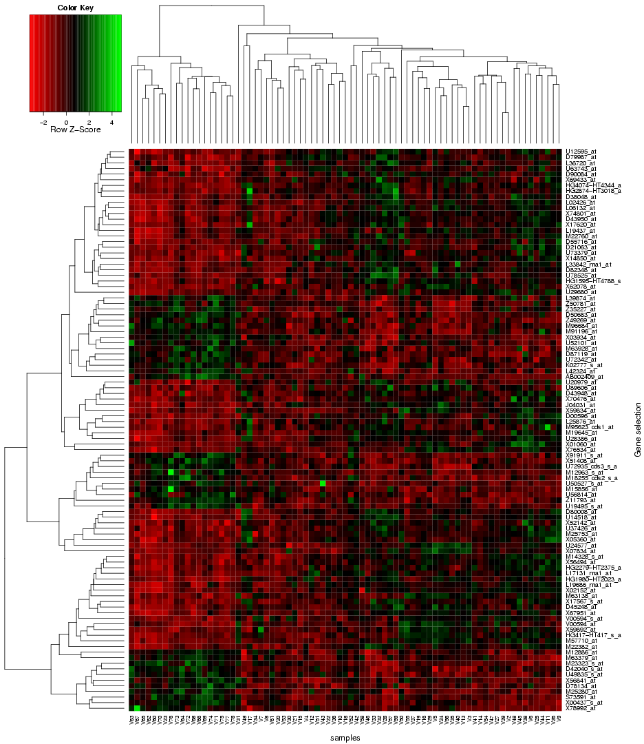
|
| Fig. 4: Heat map for differentially expressed genes extracted from microarray data and forwarded to TopoGSA |
6. Using your own interaction network as input
Although TopoGSA provides protein-protein interaction network for 5 different species (human, yeast, fly, plant, worm), we realise that some users might want to use their own network, for instance for other species or other types of molecules and relations between them (e.g. gene co-expression networks. genetic interactions).
We therefore provide a second web-interface, enabling the user to upload a network in combination with a molecule list (e.g. gene/protein list) of interest.
The data submission process consists of a simple two-step procedure:
The network file uploaded in the first step can contain molecules and relations of any type. The file format is a two-column flat-file format (also known as edge list-format), where column 1 specifies the first interactor and column 2 the second interactor (separated by a space or a tab). For example
ENSG00000000938 ENSG00000080824
ENSG00000051180 ENSG00000002016
ENSG00000179348 ENSG00000005339
ENSG00000134058 ENSG00000008128
ENSG00000072274 ENSG00000010704
...
could be the beginning of a valid network file, where all genes/proteins are in the same format. Optional comment lines in the network-file can be added by using the #-symbol as the first character in a line.
In the second step, the user has to upload the molecule list of interest (this corresponds to the gene or protein list that a user would upload on the main TopoGSA interface, when using pre-defined networks). The molecule identifiers have to match the format of the node labels in the network file to guarantee a successful mapping process. Finally, by pressing
"Start Analysis", the processing of the uploaded network will begin, and the user will be notified, when the topological properties of the network and molecule list have been computed.
The user should note that the automatic extraction, conversion and consolidation of molecule identifiers from functional annotation databases is currently not supported for arbitrary types of species and molecules. Thus, on the web-interface for user-defined networks we can only provide a comparison of subsets within the set of identifiers provided by the user. For the same reason, the automatic conversion of molecule identifiers into the format used by the network is not supported on this interface.
In order to compare subsets of identifiers, class labels have to be specified for each molecule in the uploaded identifier list (see the first section on
"Preparing and submitting your gene/protein set").
An analysis with a user-defined network will generally require more time than an analysis using the default networks, because not only the topological properties of a small subset of nodes have to be computed, but also the entire network has to be pre-processed to compute the statistics for the global network and the matched-size random subsets for the random model. For this reason, after having uploaded a network and a molecule list, the user can bookmark the webpage on which the results will be displayed after data processing, or alternatively, provide an e-mail address to obtain a notification message, when the results are available.
7. Recommended settings to solve browser compatibility issues
Depending on the user's browser and operating system, some of the dynamic or interactive features on TopoGSA (e.g. the video tutorial or the 3D plots)
might not be available without installing a browser-plugin or switching to a more common or recent version of the web-browser or operating system.
We have tested TopoGSA using the web-browsers Firefox 3.6, Internet Explorer 8.0.6 and Opera 10.50 on the operating systems Microsoft Windows XP Professional, Ubuntu Linux 9.10, MacOS X Leopard (version 10.5). The recommend screen resolution is 1280x1024. To access the 3D-plots, the user's browser
either needs to be Java-enabled (for the LiveGraphics3D-plot) or contain a VRML 2.0 plugin (for the VRML-plot).
Should you experience any layout or compatibility problems while visiting TopoGSA, we recommend that you use one of the above configurations. Also, please notify us on the contact page about any difficulties/problems you might experience with the preparation and analysis of your data.